Part I: First steps with data management

Before to start to fill network information in SHiNeMaS, it is important to setup your database with basic information. This is the topic of this first part. You will create here a new user, person, location, variable and methods. As soon as it is done we will submit your first file.

Create a new user

You are currently connected with the “admin” user which gives you the opportunity to create, modify and delete data in SHiNeMaS. But, of course, you would like to create new accounts for your colleagues, collaborators and so on. Click on the admin menu > Users and then ‘Add User’ button.

Call this user ‘rouser’ and fill a password to your convenience, click ‘Save’ and in the second step click also ‘Save’ without any modification.

Go back to the home page of SHiNeMaS, log out and then log in with the ‘rouser’. As you can see, you can’t access to the admin interface and some menu disappears. This is because you created a user with read only access. Log out and log in again with the ‘admin’ user. The user guide can give all the information to create a user with administrator access.

Create basic information: a person with a location a variable, and data descriptors

As described in the introduction John Doe and Peter Martin are already referenced in the database. Along this tutorial Steve Smith will be implied in the project. Thus, we need to record his information in SHiNeMaS. Note that a person is quite different of a user. A person is someone who is referenced in the tool who provide data, but has not necessarily a user account. A user is someone who has an access to the database and can submit/edit data if he is administrator.

To create a new person, go in Admin data > Actors & Users > Person menu. Then, ‘Add Person’ and fill the following form.

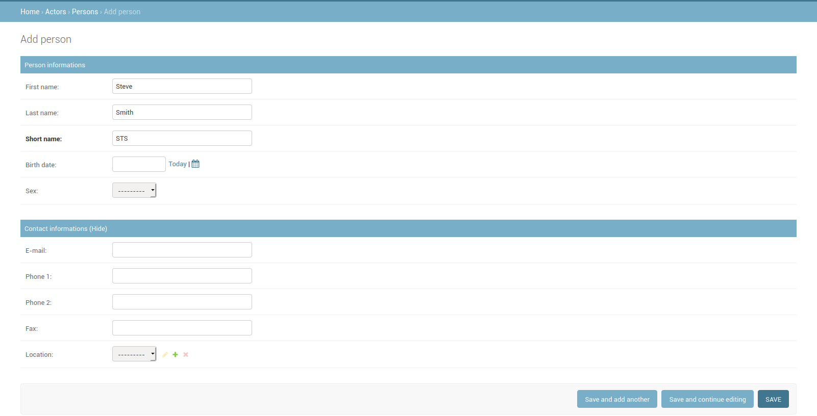
Add new person form

You are filling information about Steve Smith, but you also need information about his farm. Then you need to create a Location object (location can be a farm, an experimentation site etc.), to do it, click on the ‘+’ near the Location field and fill the form in the popup window. Use “Steve’s farm” as name and fill the short name with ‘STS’ then Save. The Location field is now filled with the one you created, you can save the person ‘Steve Smith’.

Now, we will create some few descriptors (variable, methods and reproduction methods). From the Admin data > Data Descriptors menu go in the Data variable section. As you can see some variables are already registered, click on ‘Add variable’ and fill the variable form with information name = ‘tkw’ for thousand kernel weight and choose the type ‘Type 1’ and save. This type means the data will be linked to the field plot (see user guide for more information).

If the variable defines what you measure, you need also to define how you are measuring. Still, from the Admin data > Data Descriptors menu go to Data methods. Here again some methods are already recoded, click on ‘Add method’ and fill the form with ‘method name’ = grain weight measurement, ‘unit’ = g, you can also add a description, and then save.

We also need to define some few descriptors for biological material. From the Admin data > Biological Entities go in the menu Germplasm type. Click on ‘Add Germplasm type’, and fill the form with Germplasm type = ‘Cross’ and save. SHiNeMaS is now ready to be used!

Submit a cross file

Open the ‘tutorial data’ folder you download before, you will find here a set of files that will be useful for this tutorial.

As explained in the introduction the first step will be to record the new populations created by Peter Martin. To do this, go in Prepare & Upload files > Upload files menu and fill a form with a data file, a method file, choose the type of events (cross, multiplication, diffusion etc.) and the species related to your submission. The files are ready to submit in the data folder (data file = 01-cross_2012-2013.csv and method file = 01-cross_method_2012-2013.csv), click on ‘Cross’ and select ‘Wheat’ as the species and then submit.

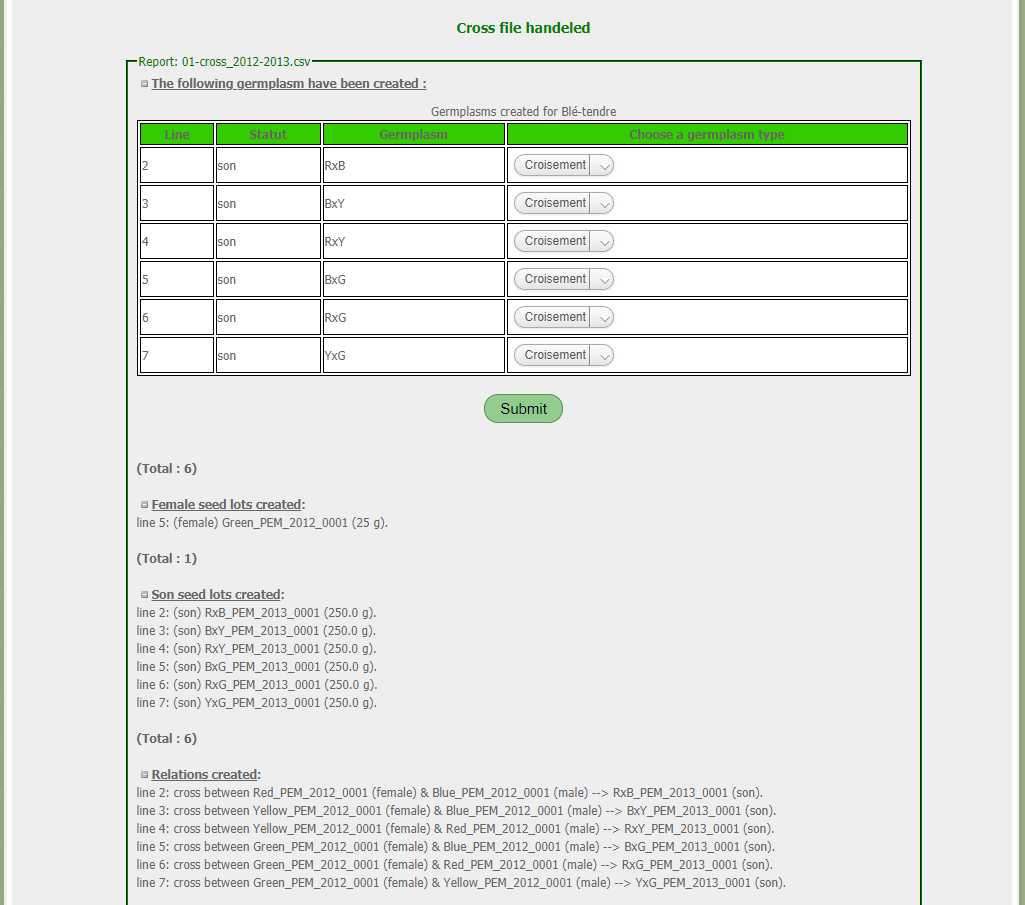
Submission report

When your submission is a success you can see report as above. Click on ‘Relations created’ to see the details. This report displays the germplasms, relations, and seeds lot that have been created. Also, you can choose a germplasm type for each germplasm newly created. Here you will select the type ‘Cross’ that you created before. As soon as ‘Cross’ is selected for each germplasm click on ‘Submit’ button.

Use the Search Bar and display a Seed lot card

If you look at the top of the web interface you can see a text field with the label ‘Search in SHiNeMaS’. This is a global search bar working with autocompleting and providing a quick access to any seeds lot, germplasm or relation card.

Search bar

In the text field start to write ‘RxY_PEM’ and then select the seeds lot ‘RxY_PEM_2013_0001’ and click on Go! The card of this seed lot is now displayed. You can have a look to it and explore information given by this card. Focus on the ‘Seed lot history’ panel, it shows how the RxY_PEM_2013_0001 seeds lot have been created. You can click on the Red_PEM_2012_0001 seeds lot and navigate in the genealogy of the lots. Obviously, there is no information in the ‘Use history’ section, but we will remedy to that in the next steps.

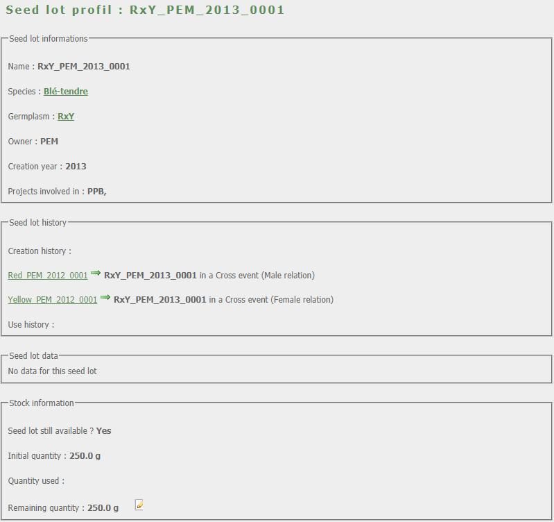
Seed lot card

Create and submit your own file

Now that the 6 populations are created, you can multiply them in 2013-2014. To do it, first use the tool to prepare files (Prepare & Upload files > Prepare files > Reproduction) and download a template file from the link on the right, get this file and put it in the ‘tutorial data’ folder. Rename it ‘02-reproduction_2013-2014.csv’. Note that the name of the file is not important for SHiNeMaS, we changed the name here just to keep a structure in data we load. In a second step, go in the menu Search > Advanced query. Use the filters ‘creation year’ = 2013 and location = ‘PEM’, select ‘Classic’ and launch the search. You should find the 6 seeds lots of the 6 populations.

Now fill your file for each column: * ‘project’ = ‘PPB’ on 6 row * ‘sown_year’ = 2013 also x6 * ‘harvested_year’ = 2014 also x6 * ‘Id_seed_lot_sown’ = copy/past the name of the seed lot one on each row * ‘intra_selection_name’ = keep empty * ‘etiquette’ = keep empty * ‘split’ = 1 on each row. It indicates that the seed lot have been divided before usage (If the whole seed lot Is used, then split=0) * ‘quantity_sown’ = 150 on each row * ‘quantity_harvested’ = put the value you want * ‘block’ = 1 * ‘X’ = 1 * ‘Y’ = 1 to 6, Y must be different on each row

In your also add the columns, this the variables we will measure

• ‘sowing_density’ = for each row put a value between 50 and 100

• ‘sowing_type’ = use value ‘mechanical’ or ‘manual’

You can save, be careful your file must be saved with a tabulated separator with no string delimiter. Usually in LibreOffice you have to check the option ‘edit filters parameters’ when you save your CSV file, and then you can choose the column separator and text delimiter. Check the documentation of your spreadsheet editor if needed. Your file is now ready, but you also need a method file. You can use the ‘00-template_methods.csv’ file, copy/paste it and rename the new file ‘02-reproduction_method_2013-2014.csv’. The rules are the same: tabulated separator and no text delimiter. You will have to row in this file for each variable you measure: * For ‘sowing_density’ variable, the type is ‘T1’ and method is ‘seeding area dentisy measurement’ * For ‘sowing_type’ variable, the type is ‘T1’ and method is ‘seeding process description’

Save your method file and go in the submission interface. Select the two files you created, check ‘reproduction’, select ‘Wheat’ and submit.

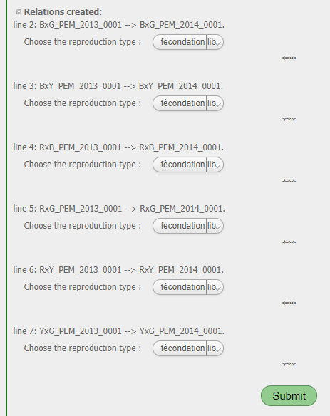
Submission report : select reproduction method

If your file was right the submission report should be displayed. As you can see on the figure above, you can select for each reproduction the ‘reproduction type’. Choose ‘open pollinated’ for each and then submit.

From the global search bar go on the card of ‘RxY_PEM_2013_0001’, now you can see that the ‘Use history’ section is filled!

You can start the next section of the tutorial !